By Sailesh Adhikari

Activity-based costing (ABC) model is a method of assigning indirect costs to products and services (Rappold, 2006).  It was first introduced in the late 1970s by the Consortium for Advanced Management- International (CAM-I) (Quesada, 2010). ABC accounting model was designed to be applicable to any kind of organization regardless of product kinds, production method, and level of automation (Andersch, et.al 2014). Kaplan and Burns (1987) describe ABC model as a more appropriate method to allocate increasing overhead cost due to advancement in technology and reduced labor-intensive work, compared to traditional costing method. Because of this, the model is widely and variously used.

ABC model is applied by obtaining the cost of each activity required to develop or produce the final product and assigning the share of the costs to unit volume of the product based on all processing activities. The first step in activity-based costing involves identifying activities and classifying them according to the cost hierarchy. Cost hierarchy is a framework that classifies activities based on the ease with which they are traceable to a product (Ainsworth et al, 2003). To allocate the costing in a process, traditional costing components are divided into four different levels as unit-level costs, batch-level costs, product-level costs, and facility-level costs (Lere 2000). This allows high fixed overhead costs to be allocated to specific activities that occur in the manufacturing process (Rappold, 2006).  Unit level activities are activities that are performed on each unit of product. Batch-level activities are activities that are performed whenever a batch of the product is produced. Product-level activities are activities that are carried out separately for each product. Facility-level activities are activities that are carried out at the plant level. The unit-level activities are most easily traceable to products while facility-level activities are least traceable (Rappold, 2006).

The main advantage of the ABC method over traditional methods is the ability to recognize different costing activity as measures of value addition instead of only considering volume or quantity of the product as in traditional costing practice (Rappold, 2006). This recognition of different costing activities helps to distribute the fixed cost evenly to each product output.  The major limitation of implementing ABC costing model in the real field is the time and knowledge of the process and model (Lere 2000). 

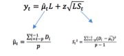
Howard (1993) developed an equation to determine the variable cost of processing individual logs into lumber which required that a variable cost function for each machine center be calculated based upon the labor costs, maintenance costs, and utility costs incurred at each machine center (Rappold, 2006). The equation proposed by Howard (1993) to determine the costing of lumber from softwood logs is:

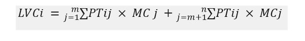
Where,

LVC = total variable cost for log “i”

PTIj = processing time for log “i” at machine center “j”

MCj = variable costs per scheduled hour for machine center “j”

m= number of machine centers with processing time function in Group 1, used to process all or part of the log “i”

n = total number of machine centers used to process all or part of the log “i”

n – m = number of machine centers with processing time functions in Group 2, used to process all or part of the log “i”

On this same model Howard (1993) defines the machines groups as follows; if the processing times of individual boards or logs can be measured for activities from any machine, they are the Group 1 machines and if it is not possible to measure the processing times for individual product for activities from any machine are Group 2 machines. The variable costs of the Group 1 machine centers are measured as a function of the individual pieces. The variable costs of the Group 2 machine centers are measured as a function of volume (Howard 1993). Howard’s equation acknowledges that not all machine centers are uniformly utilized when processing logs.

According to Garrison et. al., (1999), to implement the ABC model there may be different approach but the six core steps of costing are the major which are identified as:

Step 1: Identified activities are grouped together in activity pools

Step 2: Analysis activity identifies indirect cost and assigns it to an end product

Step 3: Based on the findings of step-1 and step-2, assign a cost to an activity pool

Step 4: Calculate activity rates for final product

Step 5: Assign the cost to cost objects with reference to identified activity pools and rates

Step 6: Prepare the costing reports

Application of ABC model to determine the hardwood and softwood CLT cost

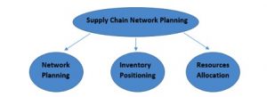
The cost of the CLT can be evaluated based on ABC model, as discuss earlier, to determine the variable cost of CLT production. The ABC model is more appropriate in this context because there will be two different products from same process that vary only in primary raw materials and each process with different raw material (may) have different functioning factor and time. To implement the ABC model, six core steps of costing implementation, as discussed by (Garrison et. Al., 1999), will be followed. The overall process of the cost evaluation is presented in Figure 1.

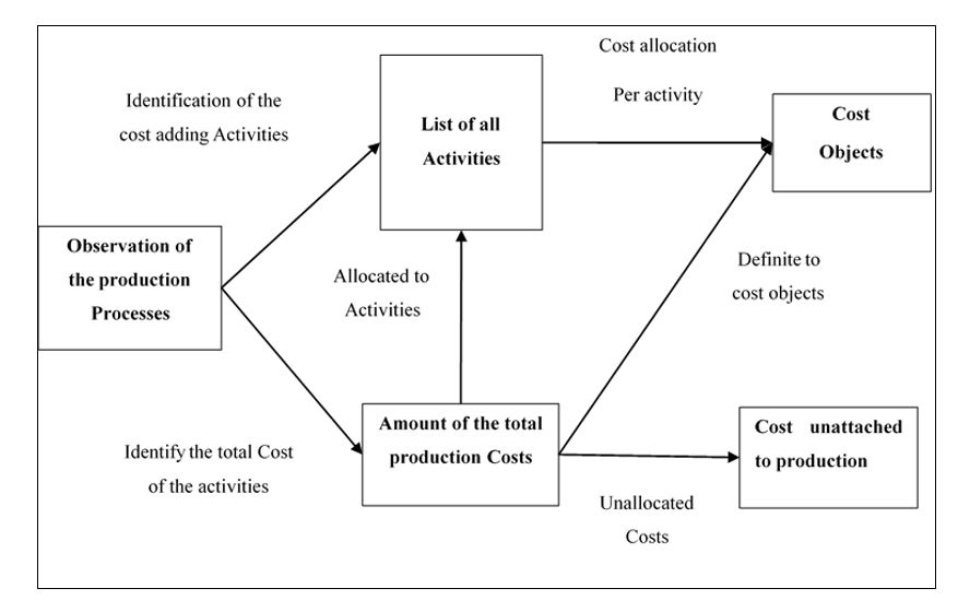
Figure 1: Purposed ABC model for product costing of CLTs.

For the cost analysis of the CLT production, all the activity that adds economic value to the product will be identified and grouped together in activity pools.  The activity pools can be studied as Unit level, Batch Level, and Product Level. The overall possible activities in the process of CLT manufacturing include but not limited to:

CLT system design cost

Raw material acquisition cost

• Direct material cost
• Purchase order cost
• Delivery cost
• CLT processing cost
• Direct labor cost
• Machine setups

Operational cost

• Primary planning and QC check cost
  • Finger jointing cost
  • Board cutting
  • Adhesive application cost
  • Pressing and drying cost
  • Trimming and edging cost
  • Quality test cost
  • CNC Processing for the architectural plans
• Product packaging cost
• Machine testing and calibration cost
• Maintenance and cleaning cost
• Transportation cost
• Installation of the CLT system
• Management cost
  • Administrative cost
  • Advertisement cost
  • Insurance/ software cost

In the second step, the activity analysis will be performed to identify total indirect costs for manufacturing CLT from both softwood and hardwood (SPF/SYP and yellow poplar). Those costs will be allocated to an end product. In the third step, the cost is allocated to an activity pool. Considering the cost of each activity pool, activity rates for the final product are calculated in the fourth step. Once activity costs, pools, and rates are identified and clearly defined, the next step is to allocate cost to cost objects. With all the information obtained, the financial report will be prepared in the final step.   The total cost of the CLT will be the sum of the cost from production to the installation of the CLT system.

References:

1. Ainsworth, P., & Deines, D. McGraw-Hill Higher Education New Product Listing: Titles due for publication April-June 2003 BUSINESS.
2. Andersch, Adrienn; Buehlmann, Urs; Palmer, Jeff; Wiedenbeck, Janice K.; Lawser, Steve. 2014. Product costing guide for wood dimension and component manufacturers. Gen. Tech. Rep. NRS-140. Newtown Square, PA: U.S. Department of Agriculture, Forest Service, Northern Research Station. 31 p
3. Garrison, Ray H., and Eric W. Noreen. Managerial Accounting. 9th ed. Boston: Irwin McGraw-Hill, 1999.
4. Howard, A. F. (1993). A method for determining the cost of manufacturing individual logs into lumber. Forest products journal, 43(1), 67.
5. Kaplan, Robert S., and W. Bruns. 1987. Accounting and Management: A Field Study Perspective. Boston: Harvard Business Publishing
6. Lere, J.C. 2000. Activity-based costing: A powerful tool for pricing. J. Bus. Ind. Mark. 15(1):23–33.
7. Quesada, H. P. (2010). The ABCs of Cost Allocation in the Wood Products Industry: Applications in the Furniture Industry. Blacksburg: College of Agriculture and Life Sciences, Virginia Polytechnic Institute and State University, PUBLICATION 420-147.
8. Rappold, P.M. 2006.Activity-based product costing in a hardwood sawmill through the use of discrete-event simulation. Ph.D. dissertation, Virginia Polytechnic Inst. and State Univ., Blacksburg, Virginia. Available at: http://scholar.lib.vt.edu/theses/available/etd-06122006-162052/. 250 pp

By Paula Fallas, dfpaula@vt.edu

In today’s conditions it is easy to think that different elements across supply chain cooperate to share information, that can potentially increase efficiency throughout the value stream. This should be true especially provided that technology can aid in such communications. Even though there is a wide range of information regarding the consequences of lack of cooperation across a supply chain it isn’t practiced regularly.

In the wood fiber supply chain, a Supplier/Consumer Relationship study conducted in 2012 showed that suppliers throughout the United States experienced a lack of cooperation between them and the customer mills. This lack of cooperation can be associated to information sharing. For example, in the Mid-South region, “suppliers cite a significant lack of joint planning that could be beneficial to both their business and the customer mills attempting to reduce costs” (Taylor, 2012). Similarly, the Southeastern region reported cooperation issues such as the lack of long-term wood orders (Taylor, 2012). Both of these concerns reflect that planning or effective demand forecasting are restricted due to the industry’s characterized business practices. The issues stated above reflect just a minimum reality of challenges to overcome.

To demonstrate the power of information sharing, it is of interest to understand and determine what the bullwhip effect is, what contributes to this effect and what are ways to decrease it.

Figure 1 shows how variability in orders fluctuate depending on each element of the supply chain. Across time both suppliers and retailers observed that even if customer demand for certain products presents low variation, orders increase in quantity and in variation moving up throughout the supply chain. The increase in variability migrating throughout each link in a supply chain is called the bullwhip effect (Simchi-Levi, Kaminsky and Simchi-Levi, 2015).

Table 1 describes the main factors contributing to the bullwhip effect.

Table 1. Main Factors contributing to the increase in variability

Demand Forecasting	Traditional inventory management techniques usually have fluctuations. Most of these techniques depend on estimates of the mean and standard deviation which depend on the quantity of data observed.
Lead Time	For example, in both safety stocks and base stock levels, the lead time and the review period are taken into consideration. This implies that a variation in lead time will in effect increase variability.
Batch Ordering	The effect of batch ordering can be easily explained through elements of the supply chain that are taking advantage of economies of scale. For example if there is a discounted price of transportation a batch will be ordered, increasing holding cost. This would be followed by a longer period without ordering. This increases variability.
Price Fluctuation	Similar to batch ordering price fluctuation stimulates stocking up when prices are low. Forward buying is used to imply that retailers purchase large quantities and small quantities depending on market conditions.
Inflated Orders	This is observed when the product is suspected to be in short supply by retailers and distributors. This generates unbalanced orders, when the period is over the standard orders are in place again.

Source: (Simchi-Levi, Kaminsky and Simchi-Levi, 2015)

The bullwhip effect can also be explained as a coordination problem between different elements of a supply chain (Moyaux, Chaib-draa and D’Amours, 2003). Therefore, how can the interactions between autonomous companies affect the bullwhip effect? More specifically how can a centralized supply chain or a decentralized supply chain affect this phenomen? A centralized supply chain is referred as a single decision maker and a decentralized is several decision makers, with different intents, interests, and information. A simplified example of Simchi-Levi et al. (2015) clarifies this question.

Considering a supply chain with a single retailer and manufacturer, where a periodic review inventory policy is implemented with a fixed lead time and a review period of 1. The order-up-to point in period t is calculated below from the demand observed, where z is a statistically obtained safety factor.

In Figure 2 the daily consumer demand and standard deviation are estimated using the moving average forecasting technique (the arrows point to both of these parameters in Figure 2). Each period (p) for which these parameters are calculated depends upon previous periods. Therefore, for each different period of time (t) the average and standard deviation are re-calculated. The consequence is each period having a different order up to level, therefore a variation in inventory is present (Simchi-Levi et al., 2015).

This model demonstrates that by increasing the lead-time (L) and decreasing p the bullwhip effect rises, under the conditions previously mentioned. In the model below the variance of customer demand is which is divided by variance of orders of a retailer (placed to a manufacturer).

With the information stated above it is intuitive to realize that without information sharing or cooperation within a supply chain the bullwhip effect increases. The manufacturer’s demand is calculated based on each previous period’s customer orders which are obtained from the retailer. These orders defer from the real customer demand. Therefore, variability can increase across the supply chain. When the demand information is known throughout each stage of the supply chain the forecasts become more accurate (Simchi-Levi et al., 2015).

Achieving coordination in a supply chain is not an easy task, and business practices in the wood industry make it more evident. Studies have been conducted in the forest supply chain to reduce the bullwhip effect. A coordination mechanism was investigated by Moyaux et al. (2013) which utilized tokens (communication resource) to communicate between autonomous agents. Figure 2 illustrates the model of the forest supply chain used in this study.

This is based on the principle that there can be two different orders communicated, using two different tokens. The first being the real time demand and the second to manage fluctuation inside the supply chain (the difference of products required by each company to maintain its inventory and the real demand). After multiple experiments a centralized supply chain with the use of tokens gives the best result, out of multiple combinations of experiments, considering total inventories, standard deviation of orders and total backorders. In general, the token based ordering is better than others Moyaux et al. (2013).

This research brings hope that better cooperation can be achieved even if full cooperation (centralized supply chain) cannot be obtained in challenging industries such as the wood fiber supply industry. Parameters that affect the variation such as lead time and forecasting methods must be improved through more cooperative relationships throughout the companies. There is still a considerable amount of work in order to achieve optimal or improved supply chains, but strategic partnerships between members is a crucial beginning.

Bibliography

• Moyaux, T., Chaib-draa, B. and D’Amours, S. (2003). Multi-Agent coordination based on tokens. Proceedings of the second international joint conference on Autonomous agents and multiagent systems – AAMAS ’03.
• Simchi-Levi, D., Kaminsky, P. and Simchi-Levi, E. (2015). Designing and managing the supply chain. 1st ed. Boston: McGraw-Hill/Irwin.
• Taylor, D. (2012). Mid-South Region Report. Supplier/Consumer Relationship Study. [online] Wood Supply Research Institute, p.6. Available at: http://www.wsri.org/tech-papers/MidSouthReport.pdf [Accessed 28 Apr. 2017].
• Taylor, D. (2012). Southeast Region Report. Supplier/Consumer Relationship Study. [online] Wood Supply Research Institute, p.6. Available at: http://www.wsri.org/tech-papers/SoutheastReport.pdf [Accessed 28 Apr. 2017].

Li Liang, email at   lli91@vt.edu

Supply chain network can be large and sophisticated, since it can involve many individual companies and many different processes and activities. Supply chain network planning is also very sophisticated, since it needs to cooperate those different individual companies and integrate many different processes and activities in the supply chain network in order to improve the value of products or minimize the system-wide costs but still satisfy the demand of customer with a good level (Che and Sha 2006). It is easy to say that the supply chain network planning can minimize cost and still maintain a good service level, but to actually achieve them both, it needs a lot of effort. Take a very straightforward example. It exists an obvious tradeoff between these two objectives, that is, if the supply chain needs to maintain a high service level, its system-wide cost will definitely increase, or if the supply chain needs to minimize its system-wide cost, the service level needs to give way. It seems that balancing the tradeoff is an art in supply chain network planning. Simchi-Levi et al (2008) stated that Supply chain network planning can help companies to:

• Balance the cost trade off among inventory, transportation, and manufacturing.
• Balance supply and demand under uncertainty through effective inventory management and positioning
• Balance the available recourses to select the most appropriate product sourcing facilities.

Associated with the above advantages, supply chain network planning can be divided in three steps as shown in Figure 1: planning, positioning and allocation. According to Simchi-Levi et al (2008), network design provides a physical configuration and infrastructure for supply chain. To achieve this objective, the data about locations of each facilities (suppliers, production plants, warehouses, distribution centers, retailers and even customers), all product information, annual demand, costs of each supply chain activities, and customer service requirements need to be collected first. After that, this huge amount of original data need to be aggregated to reduce the variance and for further utilization. The aggregated data would then be used to estimate transportation rates, mileage between two locations, warehouse costs, warehouse size, warehouse locations, service level, and future demand. The estimated data would be used to construct the supply chain network model, then both model and the estimated data would be validated by comparing the output of model with the existing data. After the validation, the model can be optimized by using mathematical optimization techniques or simulation model.

Inventory positioning is very difficult because it needs to determine the inventory control mechanism for each form of inventory (raw material inventory, work-in-process inventory, and finished product inventory), which needs to consider a lot of information. Such as production cost, distribution cost, inventory management cost, and even service level. There exist a lot of approaches for inventory management, such as (Q, R) policy, base-stock policy or critical fractile. The (Q, R) policy refers to calculate the optimal order quantity Q and reorder point R, and then place the order with a quantity of Q when inventory level reach the reorder point. The base-stock policy refers to calculate the base stock level and safety stock, when inventory level reach the safety stock level, it order up to the base stock level. The critical fractile refers to using the overage cost and underage cost to determine the optimal order quantity. Usually, the cumulative distribution function of the demand equals to the coverage cost divided by the sum of overage cost and underage cost.

Resource allocation can be done by using supply chain master planning. Master planning coordinates flows between each site and try to find the most effective way to meet demand forecast in a season cycle. It can maximize the profit or minimize the cost by balancing the demand forecasts with different capacities, and allocating production quantities to different sites to avoid bottlenecks (Stadtler 2005).

Planning the supply chain network is a very complex process but important, it involves in a set of strategic level decisions that would impact a supply chain’s future overall performance (Bahazadeh 2016). Planning of the supply network through these three steps can provide a company with a solid foundation, a better starting point, and further globally optimize supply chain performance

References:

• Babazadeh, R. (2016). Optimal design and planning of biodiesel supply chain considering non-edible feedstock. Renewable and Sustainable Energy Reviews, available online 15 November 2016
• Simchi-Levi, D., Simchi-Levi, E., & Kaminsky, P. Shankar, R. (2008). Designing and managing the supply chain: Concepts, strategies, and case studies 3^rd edition. New York: McGraw-Hill.
• Sha, D.Y., Che, Z.H. (2006). Supply china network design: partner selection and production/distribution planning using a systematic model. Journal of the operational research society. 57 (1) 52-62
• Stadtler, H. (2006). Supply chain management and advanced planning—basics, overview and challenges. European Journal of Operational Research. 163 (3) 575-588

 

 

by Gaurav Kakkar, kakkarg@vt.edu

The prospects of modernizing the use of biomass and developing cleaner liquid fuels to address concerns of energy cost, security and global warming associated with fossil fuels have led to a greater interest in Biofuels (United Nations, 2008). As classified by the UN (2008), the term biofuel means “any liquid fuel made from plant material that can be used as a substitute to petroleum-derived fuel”. International Energy Agency further adds gaseous fuels from biomass based sources to biofuels (IEA, Bioenergy, 2016). This broad term includes the familiar ones like ethanol made from sugar syrups or diesel like fuel made from plant oils to not so common ones like butanol, di-methyl ether (DME) or Fisher-Tropsch Liquids (FTL) made from lignocellulosic biomass. Moreover, as reported by IEA (2011), biofuels alone have the potential to cover up to 27% of the global transportation fuel requirements by 2050. Thus it is extremely important to understand uniform classification systems of biofuels that are globally adopted and the associated production technology. This article discuss two different classification types of biofuels based upon production technologies and biomass source.

Classification according to generations

 There are no strict technical definitions for this classification. The main distinction between them is the feedstock used and associated conversion method used. Following section discuss this classification in detail.

2. First generation: This category includes biofuels produced from conventional, well established processes. These are generally made from sugars, grains, or seeds, i.e. utilize only a specific (often edible) portion of the above-ground biomass produced by a plant. These are often produced with relatively simple processes (United Nations, 2008). Most well-known first generation biofuel is Ethanol produced from fermenting sugars extracted from starch laden crops like sugarcane, sugar beet, corn etc. Using similar processing but a different microbe for fermenting is used to make Butanol.

Pros: Mature technology, familiar feedstock, scalable production capabilities, cost competitive to fossil fuels

Cons: Food vs fuel debate, feedstock price volatility, Low land use efficiency, geographical limitations, modest net reduction in fossil fuel use and greenhouse gas emissions with current processing methods.

2. Second generation: The biofuels produced in this category are generally made from lignocellulosic biomass. This includes either non-edible residues of food crop production (e.g. corn stalks or rice husks) or non-edible whole plant biomass (e.g. grasses or trees grown specifically for energy) (United Nations, 2008). These can be produced from feedstock grown on marginal arable croplands and/or using non-food crops and residues (Biofuels Digest, 2010). These can be further classified based on conversion technology as biochemical and thermochemical. Ethanol is the most common product in this category but competitive production (without subsidies) still needs research (IEA, Bioenergy, 2016).

Pros: Surplus feedstock supply, less controversial, less dependence on geographical location, suitable for developing agrarian countries with large population.

Cons: High capital cost, technological breakthroughs needed, development of high biomass feedstocks to improve land use efficiency.

These two generations of biofuels are the most commonly addressed in academia and industry as of today. Figure 1 summarize production technologies and application of biofuels in replacing petroleum based fuel products.

First and second generation biofuels have inherent limitations preventing them to from becoming a long term alternative to petroleum. Use of food based feedstocks, competition for scare cropland and fresh water, use of fertilizers, seasonality, and population rise are few of the many (Kagan, 2010). Moreover, these fuels cannot be used above small blends without modifying the engines and have no application in Jet fuel market (a large transportation fuel segment) (Kagan, 2010; Aro, 2016). The advanced biofuels, currently is research stage, aim to fulfill this gap. They can further be divided into two generations.

3. Third generation: Biofuels made using non-arable land, based on integrated technologies that produce a feedstock as well as a fuel (or fuel precursor, such as pure vegetable oil), and require the destruction of biomass. These are similar to the 2^nd generation fuels but use lot less resources in generating feedstock. Algae is the most promising feedstock candidate in this category which cannot be matched by any other feedstock in terms of quantity or diversity (Biofuel, 2016). This category is under extensive research to reduce production costs and improve metabolic production of fuels (Aro, 2016).

Pros: Only inputs to get feedstock is CO2 and water. Less controversial, versatile array of products possible.

Cons: High capital costs, early research stage

4. Fourth Generation: This category includes biofuels which can be made using non-arable land. These do not require destruction of biomass to be converted to fuel. This technology aims at directly converting available solar energy to fuel using inexhaustible, cheap and widely available resources. They (photobiological solar fuels and electrofuels) are the most advanced biofuels currently under research (Aro, 2016).

Pros: Only inputs to get feedstock is CO2 and water. Less controversial, versatile array of products possible, least negative environmental impact

Cons: High capital costs, early research stage, long processing time. Slow yields

Food and Agricultural Organization (FAO) classification

FAO uses a comprehensive classification based on nature of feedstock and energy content rather than the conversion technology. This classification covers biofuels on the bases of origin of biomass and important trade forms. The aim to develop such system is to assist in recording trades and production stats across the globe (FAO, 2004). FAO classified biofuels into three common groups, namely, Woodfuels, Agrofuels and Municipal By-products. Figure 2 summarize the classification.

Having uniform classification systems are important both for structural innovation and future commercialization of biofuels. Moreover the classification should also be easy to understand and self-explanatory. The two major biofuel classification systems discussed above should help the reader in understanding the global biofuel commercial and underdevelopment market.

References

• Aro, E. (2016). From first generation biofuels to advanced solar biofuels. Ambio, 24-31.
• Biofuel. (2016). Third generation biofuel. Retrieved from Biofuel.org.uk: http://biofuel.org.uk/third-generation-biofuels.html
• Biofuels Digest. (2010, May 18). What are – and who’s making – 2G, 3G and 4G biofuels? Retrieved from Biofuels Digest: http://www.biofuelsdigest.com/bdigest/2010/05/18/3g-4g-a-taxonomy-for-far-out-%E2%80%94-but-not-far-away-%E2%80%94-biofuels/
• FAO. (2004). UNIFIED BIOENERGY TERMINOLOGY. FOOD AND AGRICULTURE ORGANIZATION OF THE UNITED NATIONS.
• IEA. (2011, 4 20). Biofuels can provide up to 27% of world transportation fuel by 2050, IEA report says – IEA ‘roadmap’ shows how biofuel production can be expanded in a sustainable way, and identifies needed technologies and policy actions. Retrieved from International Energy Agency: http://www.iea.org/newsroom/news/2011/april/biofuels-can-provide-up-to-27-of-world-transportation-fuel-by-2050-iea-report-.html
• IEA. (2016, 12 14). Bioenergy. Retrieved from International Energy Agency: http://www.iea.org/topics/renewables/subtopics/bioenergy/
• Kagan, J. (2010). Third and Forth Generation Biofuels: technologies, markets and economics through 2015. GTM Research.
• United Nations. (2008). Biofuel Production Technologies: Status, Prospects and Implicatiopns for trade and development. New York: United Nations Conference on Trade and Development.

 

 

 

 

 

By Paula Fallas, dfpaula@vt.edu

There is vast amount of research and information available on Lean Thinking; a management approach that incorporates a series of principals and practices to decrease waste (Czabke, Hansen, & Doolem, 2008). Key aspects for successful implementation of Lean Thinking are top management involvement and support and employee training.

Lean Thinking is not vastly applied to the forest products industry even though companies in this industry are aware of the methodology. In a survey conducted in 2010 targeting primary and secondary wood products industries Virginia findings showed that the majority of industries surveyed were aware of lean (72%) and that a lesser fraction (42%) had implemented lean initiatives (C. F. Fricke & Buehlmann, 2012). There are significant internal and external factors impacting the competitiveness of the US forest products industry such as foreign competition and higher production costs but Lean thinking could be a good strategy to overcome the lack of competitiveness of the US forest products (Czabke et al., 2008).

Implementing lean and sustaining lean is not easy (C. Fricke & Buehlmann, 2012) as it is reflected in the US Forest Products industry. The low implementation rates of Lean Thinking in the US forest products industry could translate to missing opportunities to mitigate risk from competition and to generate competitive advantages (Espinoza, Smith, Lyon, Quesada-Pineda, & Bond, 2012). According to Czabke et al. (2008), a successful implementation of lean thinking can be reached if all employees are well aligned with the lean strategy.

A key aspect in Lean Thinking implementation is to invest in people, recognizing that an educated workforce could achieve higher productivity and innovation levels (Watson, Galwey, O’Connell, & Russell, 2009). Another aspect that is very relevant when implementing Lean Thinking is to gain the support and engagement of the management (Chappell, 2002). This especially important when obstacles and difficulties arise in the implementation processes as only the determination of the managers could steer the organization towards success (C. F. Fricke & Buehlmann, 2012).

Training and education on Lean Thinking can also help to overcome challenging aspects such as resistance to change as well as communication. “Communicating, understanding, and believing in the new vision proved to be difficult, not only for employees, but also for management” (Czabke et al., 2008). The resistance of the US forest products industry towards lean can be explained by the fact that small companies tend to be reluctant towards new business trends because of the lack of funds and that they are more prone to short term planning rather then long-term planning (Westhead & Storey, 2006).

An additional important finding of the survey by Fricke & Buehlmann, (2012) showed that companies employing a Lean Manager show significant difference from the companies that don’t have one since companies with a Lean manager had a higher knowledge and resources to implement Lean. Another way that the industry can increase the success rate of lean implementation is from collaboration with universities. A related success story is Airline Manufacturing, a company that produced solid wood and plywood components. Through a change in the company’s management it was decided to collaborate with Mississippi State University and through an extension specialist the company received consultancy that helped them implement lean and even help them develop a warehouse program to track inventory (Forth, 2004). Through lean this company reduced from 5 million board feet on hand of hardwood lumber to 1 million along with achieving a reduced lead-time. Other success stories of collaboration between the industry and universities show that the industry in general was able to improve lead-time, on-time deliver, inventory turnover, and cost per unit (C. F. Fricke & Buehlmann, 2012).

In summary, the following strategies are recognized as critical steps to a successful lean thinking implementation in the US forest products industries

• Hiring of a Lean manager. The Lean manager should lead the effort and along with the management and employees, the organization needs to enter into a continuous improvement process.
• Invest in training and education of all organization’s employees. Most important asset of any organization it is its people
• The top management must commit and engage with the lean thinking implementation
• Pursue collaborations with Universities. There are a large number of support programs to industry including training, internships, and specific applied research projects.

Bibliography

• Chappell, L. (2002). Womack: Lean thinking starts with CEO. Automotive News.
• Czabke, J., Hansen, E., & Doolem, T. (2008). A multisite field study of lean thinking in U . S . and German secondary wood products manufacture.
• Espinoza, O., Smith, R., Lyon, S., Quesada-Pineda, H., & Bond, B. H. (2012). Educational Needs of the Forest Products Industry in Minnesota and Virginia in 2012. Forest Products Journal, 62(7), 613–622. Retrieved from http://login.ezproxy.lib.vt.edu/login?url=http://search.proquest.com.ezproxy.lib.vt.edu/docview/1433069442?accountid=14826
• Forth, K. D. (2004). Component Supplier Sucessful with lean methods. FDM, 79(9), 36.
• Fricke, C., & Buehlmann, U. (2012). Lean and Virginia’s wood Industry-Part II: Results and Need for Support. BioResources, 7(4), 5094–5108.
• Fricke, C. F., & Buehlmann, U. (2012). Lean and Virginia’s wood industry – Part II: Results and need for support. BioResources, 7(4), 5094–5108.
• Watson, D., Galwey, P., O’Connell, J., & Russell, H. (2009). The changing Workplace : A survey of Employers’ Views and Experiences. Employers The National Workplace Surveys 2009, 1.
• Westhead, P., & Storey, D. (2006). Management training and small firm performance: Why is the link so weak? International Small Business Journal, 14(4), 13–24.